Interesting basic PRNG distributions

by Piter Pasma

Have you ever needed a random value from a range, but you don’t want a lot of high numbers? In this article, we’ll investigate these, and other basic transformations of PRNG outputs.

The formula for a random range is lo + R() * (hi - lo), where R() is our PRNG, returning a random value between 0 and 1 (note that in some examples below, we may also use R(a), returning a random value between 0 and a). This shifts and scales the value of R() from between 0 and 1 to between lo and hi.

This means that in order to skew our random range to have (e.g.) less probability for high numbers, it is sufficient to skew the result of R() to have more probability for numbers close to 0 and less for numbers close to 1.

There are all sorts of fun formulas that transform a value between 0 and 1 into another value between 0 and 1. Such formulas are often called easing functions, and are useful for finetuning the speed of animations, among other things. We can use easing functions to transform our PRNG as well (and I recommend you to try all of them), but the possibilities are in fact broader, because we can also combine the results of several calls to R().

We’re going to use my tool the RANDOMOMETER to investigate the probability distributions generated by different formulas. The RANDOMOMETER allows you to specify the body of a Javascript function that returns a random value. When you hit ctrl-enter, it will evaluate this function many times (default is 1e6 = 1000000 times) and then draw a frequency histogram of the outputs, allowing you to see the probability distribution.

You can click on any of the formulas/histograms below to edit and view the code and histograms in the RANDOMOMETER.

Unless noted otherwise, histograms cover the range 0 to 1.

Transforming a PRNG to have less high numbers

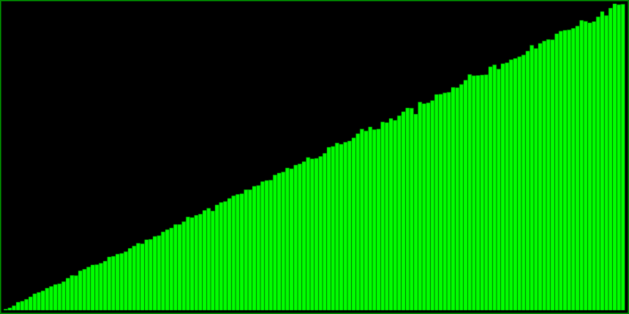
One way to do this, is to take the minimum of two random numbers:

min(R(), R())

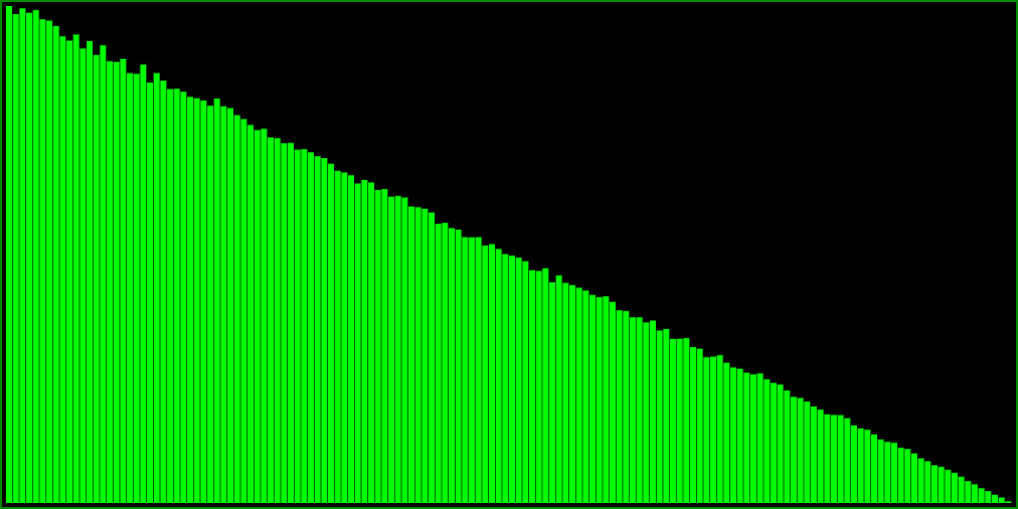
Another way to get exactly (!!) the same distribution is this formula:

1 - sqrt(R())

I think it’s interesting and fun that there are quite different formulas yielding the same distribution. Here is yet another way:

abs(R() - R())

So this is pretty cool. But as you can see from the histograms, these formulas are perhaps a little bit too skewed. The probability to return 1 goes all the way to zero (and therefore so would the probability to return the highest value in our range). What if you want something a little bit less extreme?

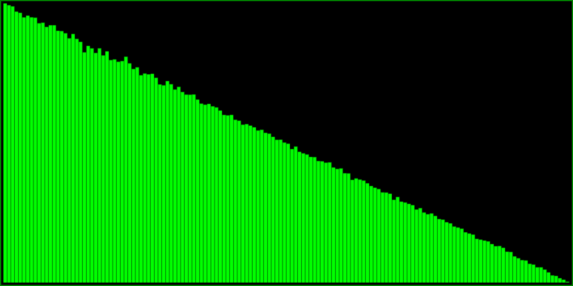
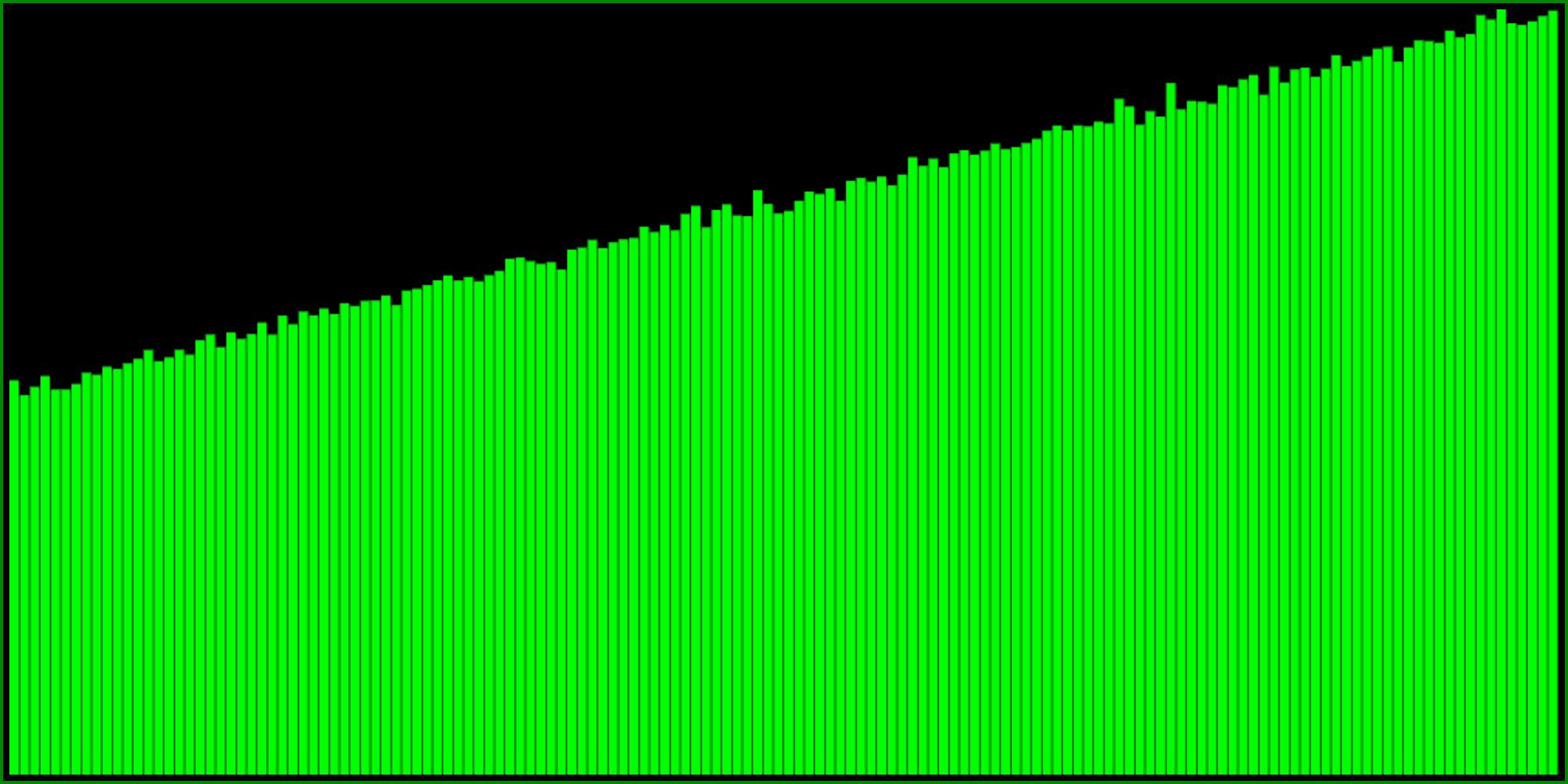
We can modify the first of the three formulas above, for instance like this:

min(R(), R(3))

This formula still returns a number between 0 and 1 (because the minimum of both is always between 0 and 1), but from the histogram it seems to have about 50% probability to return 1. Try playing with the number 3 in the above code, to see how it changes the distributions. Higher values will make it more flat, whereas lower values make the probability to return 1 smaller. Note that using values less than 1 breaks the distribution a bit because it won’t return all numbers between 0 and 1 anymore.

There’s probably a formula to calculate the required value, given a certain probability to return 1, but I haven’t quite worked it out yet. Either way, for most of my purposes it’s enough to visually estimate from the histogram by trying a few different values.

Transforming a PRNG to have less low numbers

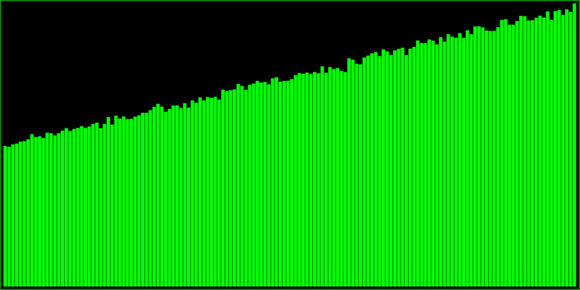
First of, we can simply do 1 - <any of the formulas above>, because doing one minus something inverts the range between 0 and 1. But we can also take the maximum of two random numbers:

max(R(), R())

And then we can do a similar modification of the formula to make it less extreme:

max(1 - R(3), R())

Note that it’s not quite as “elegant” as the min variant. So depending on your tastes for which formula looks more pretty, you might consider inverting the range of the min variant instead:

1 - min(R(3), R())

It’s actually quite easy to see that the last two formulas are equivalent, taking the “one minus” outside of the min, and because R() is the same as 1 - R() (because the uniform distribution remains the same when you invert it) and noting that min(a, b) == -max(-a, -b).

I think it’s super interesting that max(R(), R()) is equivalent to doing sqrt(R()), and I wonder if playing around with this idea might in certain other situations allow us to avoid a sqrt function, which may be more expensive than generating two random numbers.

Triangular and Normal distributions

Subtracting two random numbers from each other gives a triangular distribution centred around 0:

R() - R() (range: -1 to 1)

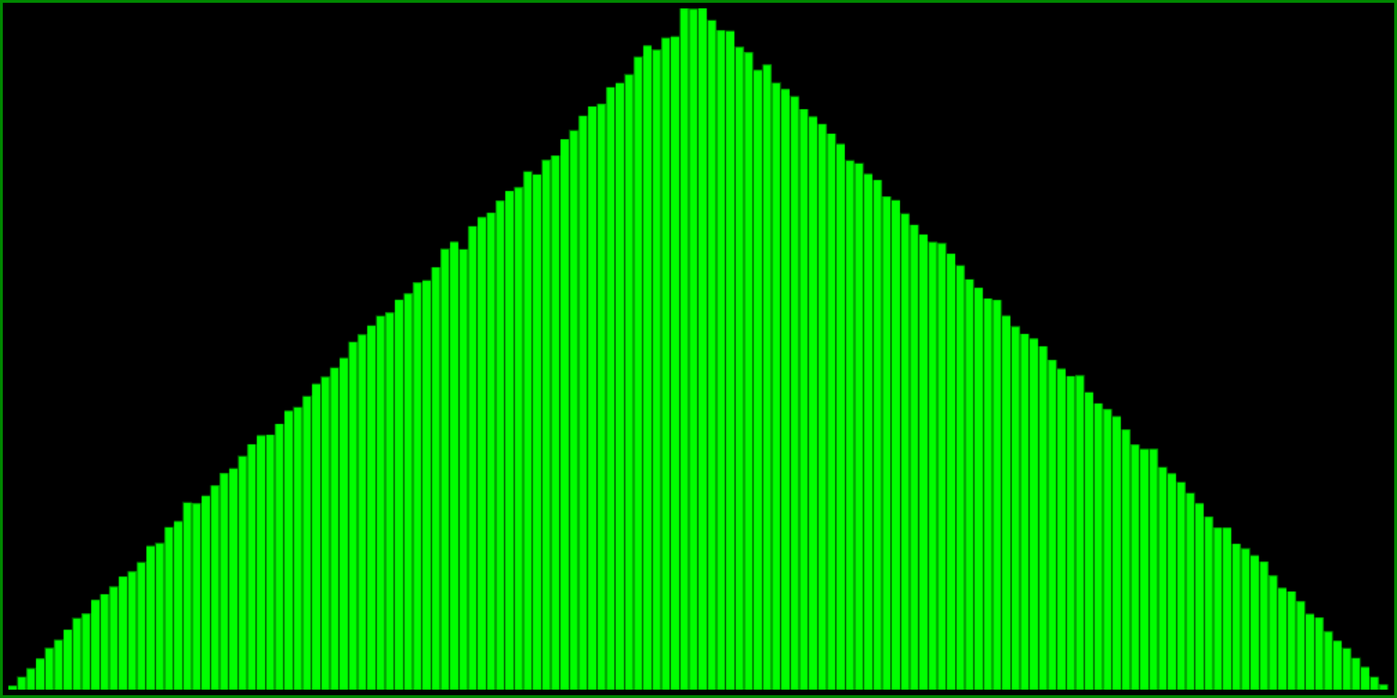
Note that the range of this histogram goes from -1 to 1. The triangle distribution is the first order (linear) approximation to the normal (or Gaussian) distribution. I use this distribution very often, scaling and adding it to a value when I want to tweak or jitter a variable around this value, with less probability for being further away from it. I usually define it as a function: T=a=>R(a)-R(a).

In general I find the triangle distribution sufficient for almost all of my normal(-ish) distribution needs. But in case you want a higher order approximation, you can try these formulas:

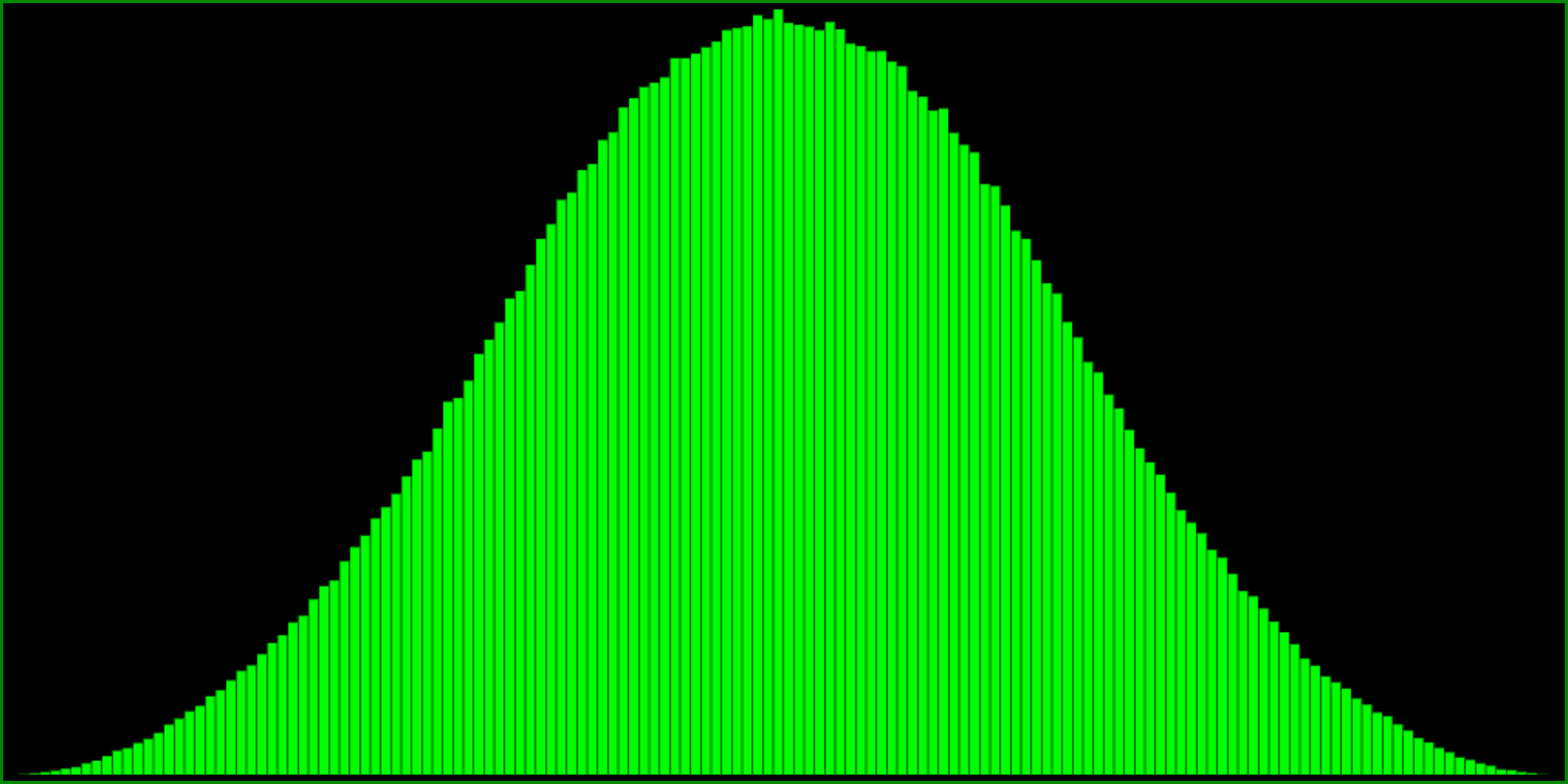
R() - R() + R() - .5 (range: -1.5 to 1.5)

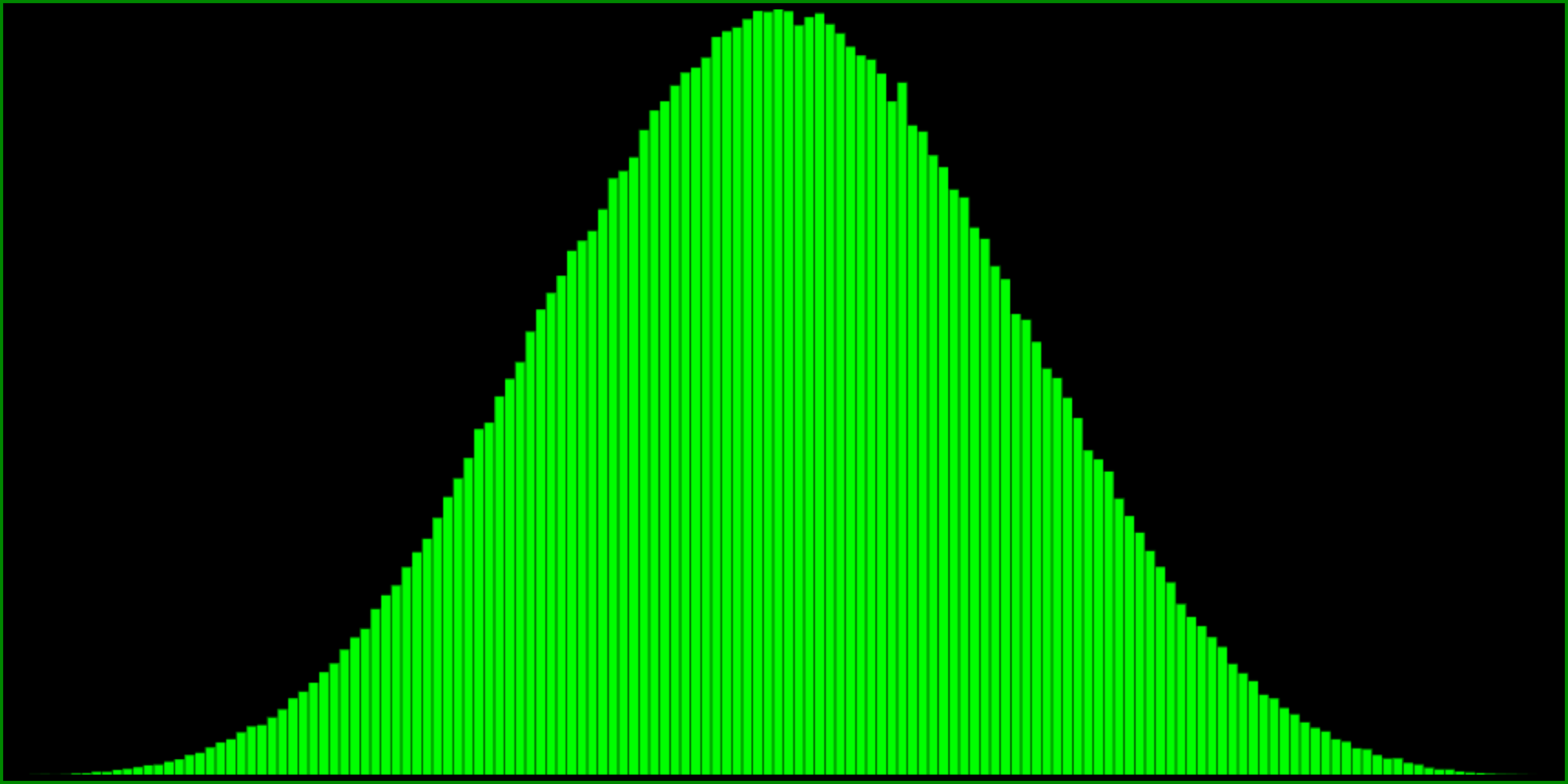
R() - R() + R() - R() (range: -2 to 2)

Note that the ranges of these histograms are -1.5 to 1.5 and -2 to 2, respectively. I’m not exactly sure what their standard deviations are.

If you need an even better approximation to the normal distribution, you could keep adding and subtracting more and more random numbers, and this would work. I think it converges pretty quickly actually. However, at some point generating that many random numbers probably gets less efficient than doing the Box-Muller transform (which actually gets you two independent normally distributed values at once).

Other fun stuff

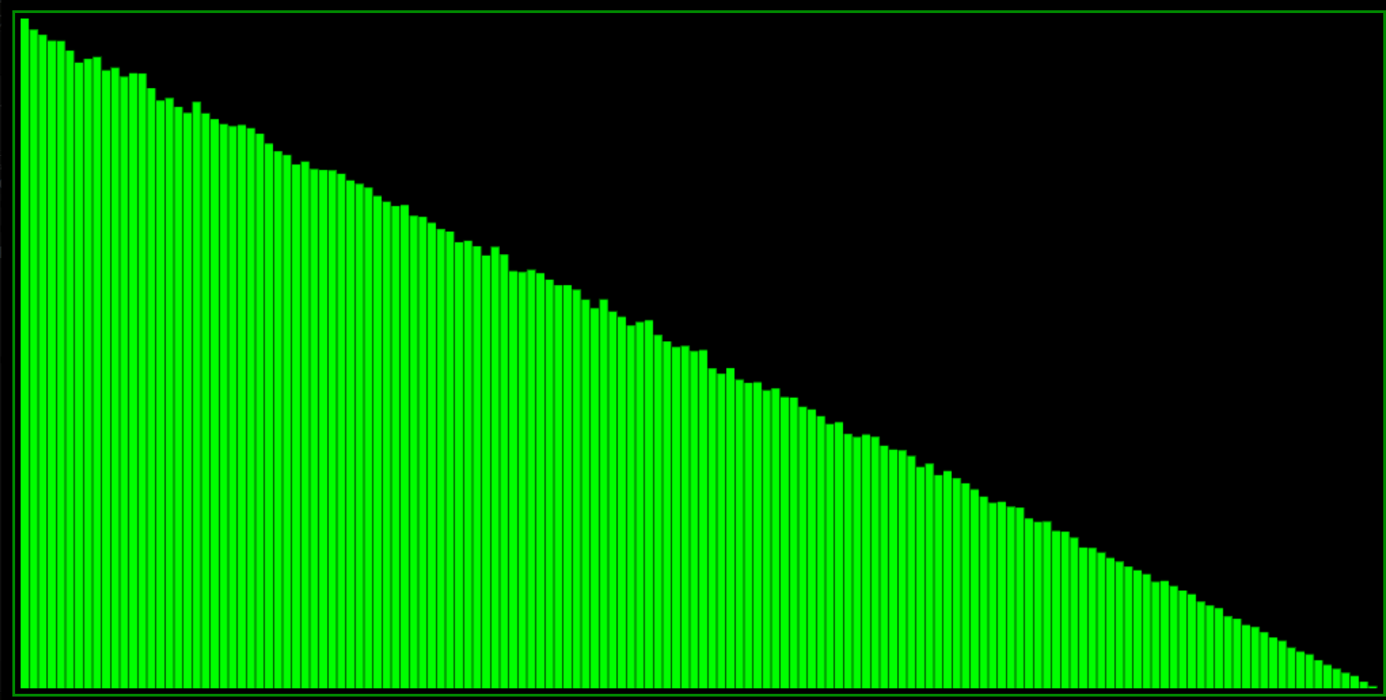
One of the most basic easing functions is x * x, squaring a number between 0 and 1 always yields another number between 0 and 1. Trying this in our RANDOMOMETER looks like this:

R()**2

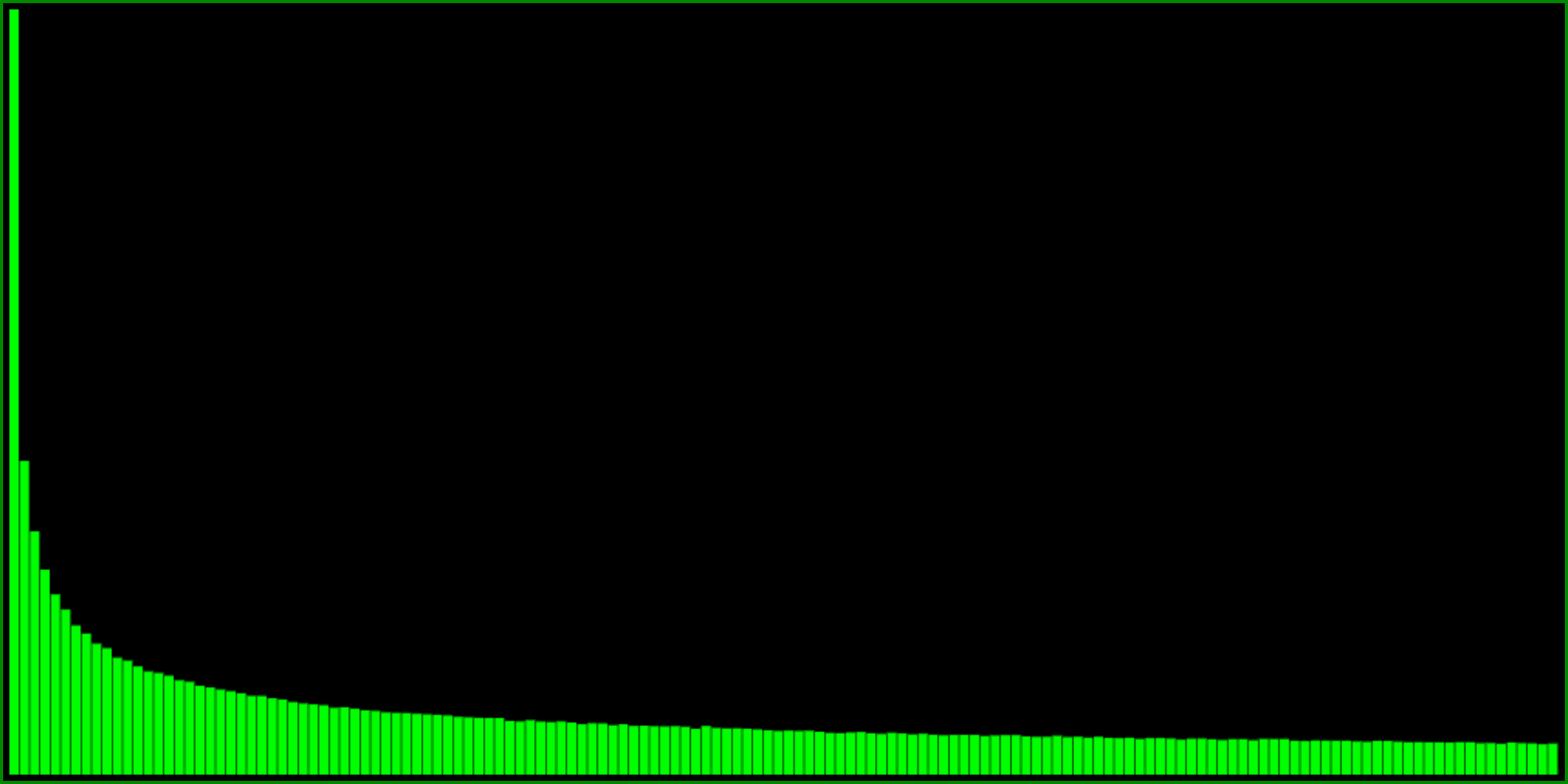
Note that the probability distribution is really steep, yet doesn’t reach a probability of 0 at one.

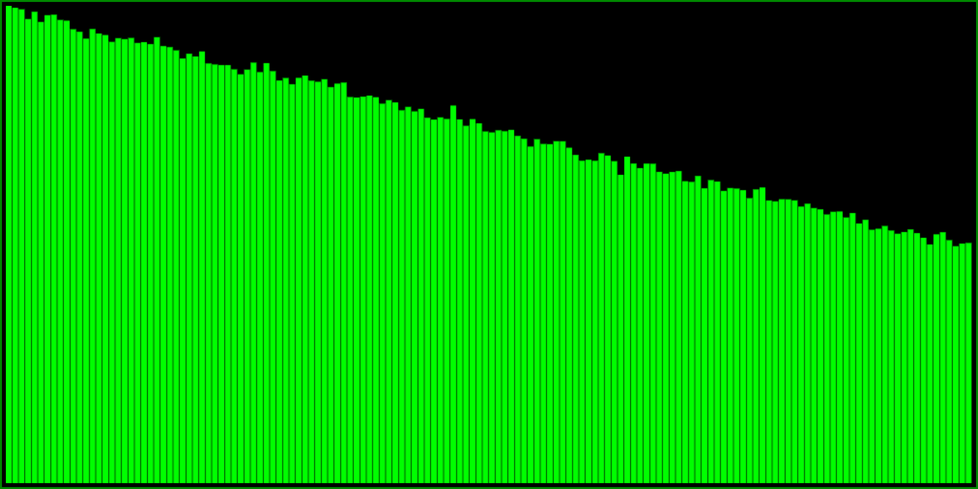
Instead of squaring one random number, we can also multiply two different random numbers. If you think about it, this is not quite the same, but what does the histogram look like?

R() * R()

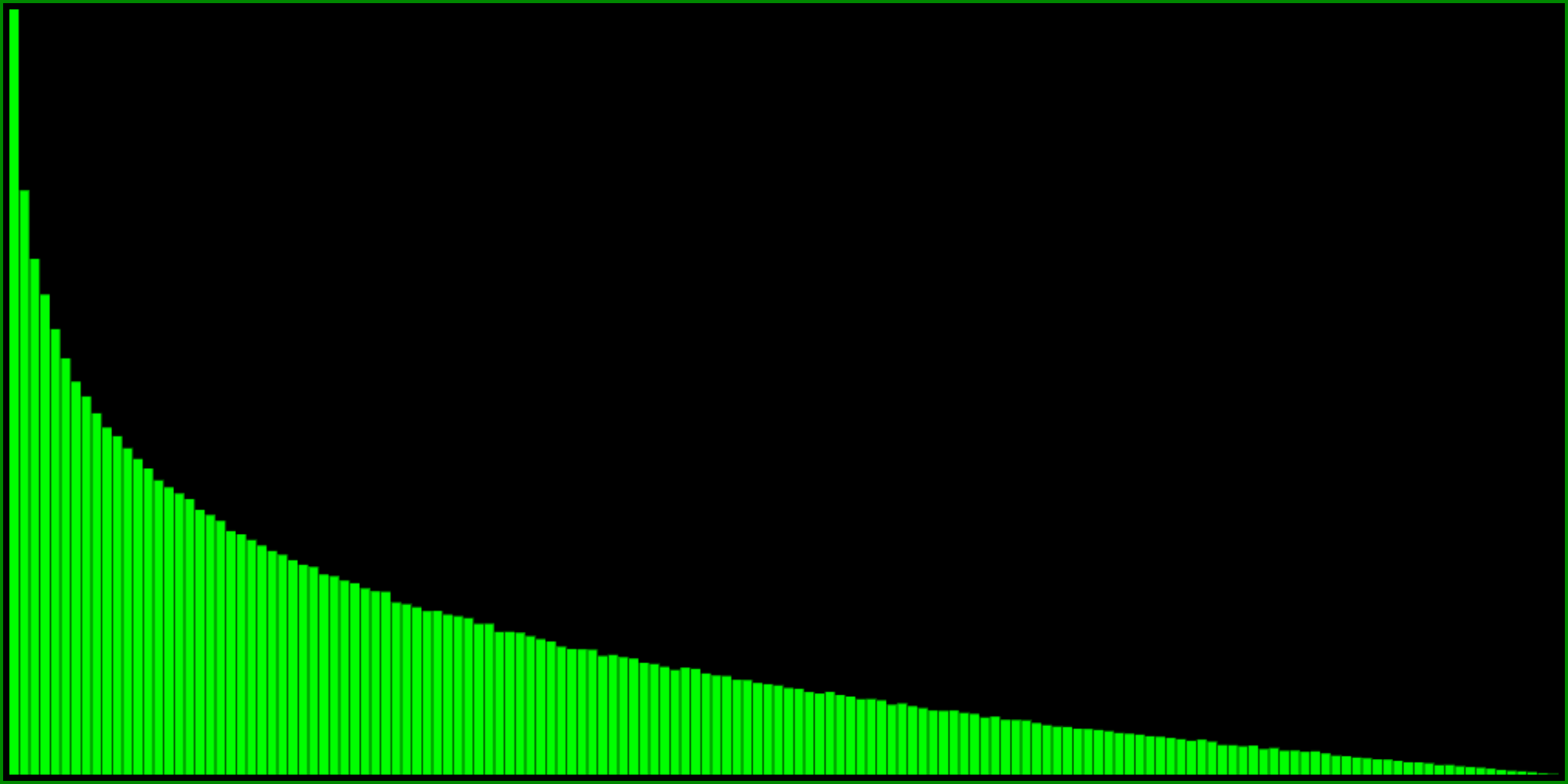
This probability distribution is still steeper than say, min(R(), R()), but not quite as steep as R()**2. Also note that unlike the previous it does have 0 probability at one. When I need a steep distribution, this is the one I usually reach for.

Experiment!

You can combine the above ideas in all sorts of fun ways to generate even more different probability distributions.

What would happen if you raised R() to different powers?

Or if you took the minimum of three random numbers? Or the maximum? What about taking the middle one?

Please experiment and do let me know if you find anything cool!

Maybe I’ll add more related links, but I wanted to link this one article from extremelearning.com.au which is a super cool blog. This particular article is relevant in case you ever need to generate uniform points on a sphere, inside a ball or a disc, on or in any N-dimensional sphere or ball. Even if you think you know how to do this, it might list a couple of methods you haven’t heard about, so check it out in case this interests you: